|
COMPLEXITY INTERNATIONAL |
| ISSN 1320-0682 |
| Source: | http://life.csu.edu.au/complex/ci/vol6/andresen/ | Received: | 01/07/1998 | ||
| Vol 6: | Copyright 1998 | Accepted for publication: | 15/10/1998 |
Trond Andresen
Department of Engineering Cybernetics,
The
Norwegian University of Science and Technology,
N-7034 Trondheim,
NORWAY.
Email: Trond.Andresen@itk.ntnu.no
Real-world stock markets are volatile and expresses such traits as overvaluation, psychological moods, cycles and crashes. This paper develops and explores a fairly simple model which expresses these traits. The model is continuous and non-linear. It is developed in stages. In the initial stages it applies to the price dynamics of one type of stock only. Later on it is applied to a weighted price index of different stocks, to try to capture the dynamics of a stock exchange as a whole. The model is not based on micro individual agents, but on the market as a whole displaying composite behavior that is argued to be the aggregate result of individual agent behaviour. The idea is to make some behavioural assumptions, and then adjust parameters and explore whether realistic qualititative traits of stock market dynamics show up. From this follows that the model can make no claims whatsoever to predict when and how much a given stock market will rise or fall. Its purpose is instead to gain qualitative insights into the mechanisms of stock market behaviour.
This paper is a systems engineer's attempt to understand and construct a model of stock market dynamics. The model is generic, i.e. it is not an attempt to model or predict the behaviour of a specific stock exchange. The main assumptions behind the paper are as follows:
It is considered a fact of life that a significant share of stock market behaviour consists of following the herd, ``noise trading'', ``trend chasing'', ``technical trading'' etc. Thus we do not engage in the discussion of ``how can such stock market agents prevail, won't they be weeded out since they are non-rational?'', as for instance in DeLong et al. [1]. Instead we hold that non-rationality is a an observable trait of real-world stock markets. This is in the tradition of J. M. Keynes [2], who states: ``...all sorts of considerations enter into the market valuation which are in no way relevant to the prospective yield'' (p.152), ''...It might have been supposed that competition between expert professionals... would correct the vagaries of the ignorant individual...However, ...these persons are, in fact, largely concerned, not with making superior long-term forecasts of the probable yield of an investment over its whole life, but with foreseeing changes in the conventional basis of valuation a short time ahead of the general public...For it is not sensible to pay 25 for an investment of which you believe the prospective yield to justify a value of 30, if you also believe that the market will value it at 20 three months hence.'' (pp.154-55), ``...The social object of skilled investment should be to defeat the dark forces of time and ignorance which envelop our future. The actual, private object of most skilled investment today is to beat the gun, as the Americans so well express it, to outwit the crowd, and to pass the bad, or depreciating, half-crown to the other fellow.'' (p. 155).
We also assume that there exist ``fundamentals'', or an ``anchor'' stock price corresponding to a sustainable yield - a yield that is also ``reasonable'', compared to alternative financial instruments like bonds. Furthermore, it is assumed that the aggregate of agents have some sort of feeling for what these fundamentals are (at least when stock prices are far away from them), and that this is crucial for long-range stock market dynamics. This is at odds with Davidson [3], who holds that any stock price is just as likely to prevail as another, based on the view that the future is completely unpredictable at any instant in time.
The model is of the top-down category, thus not based on a population of ``micro'' individual agents in the artificial life tradition. It is of a continuous non-linear differential equation type, of the market as a whole, displaying composite behaviour that is argued to be the aggregate result of individual agent behaviour.
This paper is quite different from that of for instance W. Brian Arthur et al. [4], both in its top-down paradigm, and in important behavioural assumptions. Arthur et al. conclude that small bubbles and crashes will occur (how often is not clear since they in their paper do not put any scale on the time axis) because agents occasionally, because of willingness to experiment, will lock onto each other in bubble-like excursions away from a ``correct'' price that would otherwise follow from a pure rational expectations scenario. Related to Arthur et. al. is a paper of Brock and Hommes [5], who argue that price volatility is due to agents choosing ``cheap'' but destabilizing trading strategies near the correct price, but more expensive, better and stabilizing (thus moving the price towards the correct level) strategies when prices are obviously off the mark. Common for both papers is the view that dynamics and volatility can be explained solely through endogenous mechanisms and a basically ``rational'' type of agent behaviour. This paper, as stated above, assumes that agents have significant irrational behaviour traits, and furthermore that dynamics are also a consequence of exogenous inputs in the form of events and mood changes.
The large differences in approaches to stock market modeling are understandable. Agent behaviour in a stock market is extremely complicated and heterogeneous. Any such model must because of necessary and strong simplification be fairly speculative. Therefore several angles of attack on this problem should be explored, and this paper is one such attempt.
The dynamics of the market are considered to be driven by three main demand components: One due to the market's valuation of the firm's real-economic prospects (the ``anchor'' value of the stock, see above), another due to short-term herd mentality (over minutes and hours),and a third due to long-term public mood shifts (over several years).
The model's dynamics stem mainly from these internal feedback loops, but the market is also assumed to be driven by a sequence of exogenous stochastic ``event pulses''. This pulse process accounts for both changes in macroeconomic conditions (for instance a change in interest rates), fresh information about different firms (news about quarterly earnings and similar), and individual agents taking action for some exogenous reason (as opposed to ``bandwagon'' - or other endogenously based decisions).
The model will be developed in four stages:
The presentation is based more on block diagrams than (equivalent) (differential) equations. This choice follows from a conviction that insights into feedback effects and dynamics come much easier this way.
Consider the block diagram in figure 1.
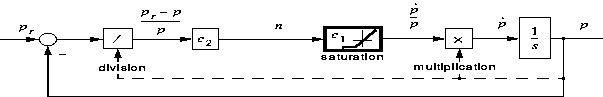
Figure 1: A ``rational'' market
Figure 2: exponential response-``rational market''
The symbols in the diagram are defined as follows (denomination is shown in brackets, empty brackets means that the corresponding entity is dimensionless):
![]() = Real or sustainable value of the stock [ ], expressed
by the price/earnings ratio it can yield in the long run. At
= Real or sustainable value of the stock [ ], expressed
by the price/earnings ratio it can yield in the long run. At ![]() the stock is neither over- or undervalued. For convenience we will use the term
``price'' or ``value'' in the following, even if we are talking about the
p/e ratio.
the stock is neither over- or undervalued. For convenience we will use the term
``price'' or ``value'' in the following, even if we are talking about the
p/e ratio.
p = current market price (i.e. p/e ratio) of stock [ ].
![]() = per cent change in price per day [% / day]. The dot
implies differentiation.
= per cent change in price per day [% / day]. The dot
implies differentiation.
s = differentiation operator [![]() ].
].
n = net current demand for stock [number of units]. This demand may be negative, i.e. when there is a net surplus of stocks offered.
![]() = constant factor [% / (number of units
= constant factor [% / (number of units day)] transforming net demand into price increase
rate. The total number of stocks issued is incorporated in this factor. There
is, as indicated in the figure, saturation in price decrease rate, since the
surplus offered cannot exceed the total number of stocks issued. In the model,
this is translated into a maximum rate of price decrease.
day)] transforming net demand into price increase
rate. The total number of stocks issued is incorporated in this factor. There
is, as indicated in the figure, saturation in price decrease rate, since the
surplus offered cannot exceed the total number of stocks issued. In the model,
this is translated into a maximum rate of price decrease.
![]() = constant factor [number of units / %] transforming
relative price deviation into corresponding net demand. The total number of
stocks issued is incorporated also in this factor.
= constant factor [number of units / %] transforming
relative price deviation into corresponding net demand. The total number of
stocks issued is incorporated also in this factor.
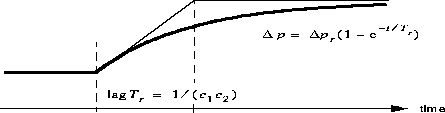
The model in figure 2 is a simple first order non-linear differential equation,
which holds above the negative saturation limit for ![]() .
If we consider only the dynamics from
.
If we consider only the dynamics from ![]() to p, the system is
linear within saturation limits. But we stick to the non-linear formulation
since we need to access surplus demand n at later stages.
to p, the system is
linear within saturation limits. But we stick to the non-linear formulation
since we need to access surplus demand n at later stages.
A rational market implies that all agents have the same perfect information
about ![]() . Any change in
. Any change in ![]() is responded to by each agent in the same manner. However, action is here
assumed to be dispersed in time. At this stage we assume that agents receive
perfect information, but they do not receive it simultaneously, or act
instantaneously after receiving it. It follows from (1) that the
time span needed for price adjustment is inversely proportional to the factors
is responded to by each agent in the same manner. However, action is here
assumed to be dispersed in time. At this stage we assume that agents receive
perfect information, but they do not receive it simultaneously, or act
instantaneously after receiving it. It follows from (1) that the
time span needed for price adjustment is inversely proportional to the factors
![]() and
and ![]() . If we now consider the case
of a stepwise increase in
. If we now consider the case
of a stepwise increase in ![]() , for instance because a
technological breakthrough has occurred in the firm, then the resulting price
adjustment path is a first order stable exponential step response as shown in
figure 2.
We have no overshoot, no oscillations, no unpredictable excursions, just a
smooth and asymptotically perfect price adjustment. This is of course a
completely unrealistic representation of what occurs in the real world. At the
same time, it should be noted that this is the way a stock market ought
to work, reflecting real-economic changes impacting the listed firms, and
nothing else.
, for instance because a
technological breakthrough has occurred in the firm, then the resulting price
adjustment path is a first order stable exponential step response as shown in
figure 2.
We have no overshoot, no oscillations, no unpredictable excursions, just a
smooth and asymptotically perfect price adjustment. This is of course a
completely unrealistic representation of what occurs in the real world. At the
same time, it should be noted that this is the way a stock market ought
to work, reflecting real-economic changes impacting the listed firms, and
nothing else.
At this stage we introduce two new phenomena. The first is that individual agents act upon imperfect and differing information. Depending upon whether he or she overvalues or undervalues the stock, the agent will demand too much or to little, compared to what demand would have been, based on a correct valuation. We assume that the distribution of erroneous information over all agents - also when accounting for agents' different influence in the market - is such that the mean of aggregate erroneous demand is zero, and that the demand error follows a normal distribution around this zero mean. We also assume that individual agents' errors in demand change with time. The choice is then to model aggregate demand error as a zero-mean normally distributed stochastic process (more on what sort of process later on).
The second phenomenon is the ``bandwagon'' effect. We explain this by referring to a block diagram of a stage 2 model, shown in figure 3:
Figure 3: A market with bandwagon effects
Surplus aggregate demand is now assumed to consist of three components,
We have
![]() = Demand component due to agents being informed about the
sustainable value of the stock.
= Demand component due to agents being informed about the
sustainable value of the stock.
![]() = Component due to agents watching price
increase/decrease rate and doing ``technical trading'' based on this. The
sustainable value of the stock has no direct influence on this component.
Subscript b signifies ``bandwagon''.
= Component due to agents watching price
increase/decrease rate and doing ``technical trading'' based on this. The
sustainable value of the stock has no direct influence on this component.
Subscript b signifies ``bandwagon''.
![]() = Component due to agents having different and erroneous
information about the sustainable value of the stock. This is the zero mean
stochastic process discussed above. Subscript e signifies ``error''.
= Component due to agents having different and erroneous
information about the sustainable value of the stock. This is the zero mean
stochastic process discussed above. Subscript e signifies ``error''.
Furthermore, we have introduced a transfer function ![]() in figure 3.
This function decides the speculative component of market behaviour. There is a
positive feedback through
in figure 3.
This function decides the speculative component of market behaviour. There is a
positive feedback through ![]() from price increase rate to
the surplus demand component
from price increase rate to
the surplus demand component ![]() . If for instance
. If for instance ![]() is large and positive at a certain moment, many agents will jump
on the bandwagon and buy now with the hope that prices will continue to rise. Of
course some technical trading strategies are more elaborate than this, for
instance action in counter-phase, i.e. buying when prices are falling
in the expectation that they will rise later on. It is assumed however, that
herd mentality is the dominant type of speculative behaviour. Involving Occam's
razor, the simplest transfer function that accounts for this, is
is large and positive at a certain moment, many agents will jump
on the bandwagon and buy now with the hope that prices will continue to rise. Of
course some technical trading strategies are more elaborate than this, for
instance action in counter-phase, i.e. buying when prices are falling
in the expectation that they will rise later on. It is assumed however, that
herd mentality is the dominant type of speculative behaviour. Involving Occam's
razor, the simplest transfer function that accounts for this, is
Here ![]() expresses the small time lag from acquiring price
information to buying (or selling), that speculative action cannot get around.
This lag is due to delays in acquiring information, considerations, and then
getting the trading done. The gain
expresses the small time lag from acquiring price
information to buying (or selling), that speculative action cannot get around.
This lag is due to delays in acquiring information, considerations, and then
getting the trading done. The gain ![]() expresses how strong
speculative action is, based on the available price change rate information.
expresses how strong
speculative action is, based on the available price change rate information.
Note that we say ``action'', not ``agents''. Individual agents may of course operate in a purely speculative or herd mode, others may again be pure ``real investors''. But most have composite motives (real-economic more or less off the mark, and speculative). When the market as a whole is considered, however, this discussion becomes uninteresting, since the market as a whole must necessarily have a ``composite motive''.
As already stated, the surplus demand component ![]() accounts for the aggregate effect of agents making erroneous and different
assumptions about the stock value, but in such a way that the mean error in
surplus demand is assumed to be zero. We now also incorporate the effects of
differences in individual speculative behaviour into this noise process, since
in reality each speculative agent will act according to a unique transfer
function. It will not be linear and it will be complex, and its parameters and
even structure will change with time. We have averaged out all this individual
behaviour into the transfer function (3). We then
posit that what is lost through this simplification may be assumed to be to a
sufficient degree represented in the error process
accounts for the aggregate effect of agents making erroneous and different
assumptions about the stock value, but in such a way that the mean error in
surplus demand is assumed to be zero. We now also incorporate the effects of
differences in individual speculative behaviour into this noise process, since
in reality each speculative agent will act according to a unique transfer
function. It will not be linear and it will be complex, and its parameters and
even structure will change with time. We have averaged out all this individual
behaviour into the transfer function (3). We then
posit that what is lost through this simplification may be assumed to be to a
sufficient degree represented in the error process ![]() . Thus this process is assumed to have two origins: Erroneous estimates of the
stock's sustainable value, and modeling errors due to aggregation of the
speculative (bandwagon) feedback path.
. Thus this process is assumed to have two origins: Erroneous estimates of the
stock's sustainable value, and modeling errors due to aggregation of the
speculative (bandwagon) feedback path.
If we now consider a situation where the price of the stock is at its sustainable value, the market will have no real-economic incentive to trade. But trading will take place all the same. Individual more or less rational, more or less well-informed agents have their own assessment, and they trade also in this situation. In the language of our model, we may say that the error process is an exogenous input or disturbance that excites the system, so that the market is never in equilibrium, but fluctuates around it.
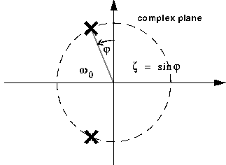
The model in figure 3 is non-linear. But if we consider small fluctuations around a constant sustainable value , it may be approximated by a linear model, see figure 4.
Figure 4: A linear model
Figure 5: Eigenvalues of linear model
Since fluctuations are assumed to be small, we may ignore the saturation. And
the blocks with division and multiplication in figure 4
may now be swapped with respectively constants ![]() and
and ![]() . We have a linear system which is excited by the error
process
. We have a linear system which is excited by the error
process ![]() . The transfer function from
. The transfer function from ![]() to p is
to p is
where the undamped resonance frequency is
and the relative damping factor is
The two eigenvalues of the system are indicated in figure 5.
Consider a case where ![]() is increased while
is increased while ![]() is held fixed, i.e. speculative action is stronger while
the information/decision time lag remains the same. From (5) we see
that
is held fixed, i.e. speculative action is stronger while
the information/decision time lag remains the same. From (5) we see
that ![]() is independent of
is independent of ![]() , while
, while ![]() decreases with increasing
decreases with increasing ![]() . In terms of figure 5,
this means that the eigenvalues of the system move along the circle towards the
imaginary axis. The system approaches the border of instability, which in the
language of the market translates as increased volatility: For a given variance
in the error process
. In terms of figure 5,
this means that the eigenvalues of the system move along the circle towards the
imaginary axis. The system approaches the border of instability, which in the
language of the market translates as increased volatility: For a given variance
in the error process ![]() , the variance in price will
increase with
, the variance in price will
increase with ![]() .
.
Figure 6: Impulse response in price due to bandwagon feedback
Figure 7: Eigenvalues move with increasing
Figure 6
shows responses of the system to a small and short error process pulse, i.e.
where some agents suddenly demand a certain amount of stock, even if the initial
price is equal to the anchor value ![]() . The amplitude of the pulse
is 500 units of stock demanded out of 10.000. The pulse lasts 5 minutes,
corresponding to 1/78 of a trading day of 6.5 hours. (The 6.5 hour trading day
is equal to that of the New York Stock Exchange).
. The amplitude of the pulse
is 500 units of stock demanded out of 10.000. The pulse lasts 5 minutes,
corresponding to 1/78 of a trading day of 6.5 hours. (The 6.5 hour trading day
is equal to that of the New York Stock Exchange).
The figure shows three price responses to this pulse, with parameters ![]() =constant, and
=constant, and ![]() . Following (6), these
values for
. Following (6), these
values for ![]() correspond to decreasing gain
correspond to decreasing gain
![]() .
.
In figure 6
- as opposed to figure 2
- the responses are from simulations where numerical values for system
parameters have been chosen. This has been done by the following procedure:
First, we choose a total number of stocks issued =10.000, and a sustainable
stock value ![]() . We may choose these values
freely; the choices do not make any difference for the analysis to follow.
. We may choose these values
freely; the choices do not make any difference for the analysis to follow.
We assume that when all 10.000 units are demanded, respectively offered, on
the market, this corresponds to a price change rate of ![]() % per day. This decides the coefficient
% per day. This decides the coefficient ![]() . The lower saturation occurs for
. The lower saturation occurs for ![]() .
.
We then set ![]() and are back to the stage
one model. Only rational trading decisions are made, and we may posit some
adjustment lag (see figure 2).
We choose
and are back to the stage
one model. Only rational trading decisions are made, and we may posit some
adjustment lag (see figure 2).
We choose ![]() [days], on the basis that
such decisions are more carefully considered than technical trading decisions
(see below), which are taken during fractions of a single day.
[days], on the basis that
such decisions are more carefully considered than technical trading decisions
(see below), which are taken during fractions of a single day.
Since we have now chosen both ![]() and
and ![]() ,
and
,
and ![]() (see figure 2),
we get
(see figure 2),
we get ![]() .
.
It now remains to decide the parameters ![]() and
and ![]() . Aiming for realism, we want the price dynamics due to
the bandwagon loop to be very fast, in the order of a fraction of a day. And
there should be at least one distinct overshoot (i.e. some volatility)
before the response settles down.
. Aiming for realism, we want the price dynamics due to
the bandwagon loop to be very fast, in the order of a fraction of a day. And
there should be at least one distinct overshoot (i.e. some volatility)
before the response settles down.
We start by choosing ![]() such that one day
corresponds to fifteen full undamped (
such that one day
corresponds to fifteen full undamped ( ![]() ) oscillations, see figure 6.
When damping is increased to
) oscillations, see figure 6.
When damping is increased to ![]() , we get the impulse
response delineated in bold in figure 6.
We have some overshoot, indicating a certain amount of volatility. This is our
choice for the dynamics of the bandwagon loop. The initial price response pulse
due to technical traders jumping on the bandwagon lasts approximately 0.03
trading days = 12 minutes, and the reaction dies out after around 30 minutes.
From the choice of
, we get the impulse
response delineated in bold in figure 6.
We have some overshoot, indicating a certain amount of volatility. This is our
choice for the dynamics of the bandwagon loop. The initial price response pulse
due to technical traders jumping on the bandwagon lasts approximately 0.03
trading days = 12 minutes, and the reaction dies out after around 30 minutes.
From the choice of ![]() ,
, ![]() the corresponding pair
the corresponding pair ![]() ,
, ![]() is calculated from (5) and (6). (See
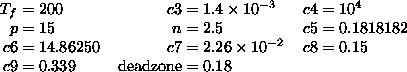
end of paper for complete list of parameter values.)
is calculated from (5) and (6). (See
end of paper for complete list of parameter values.)
At this stage, we emphasize that the above, and later, choices of parameter values, must necessarily be somewhat arbitrary. Our defense is that simulation experiments have demonstrated that similar qualitative system behaviour shows up under a fairly wide spectrum of values.
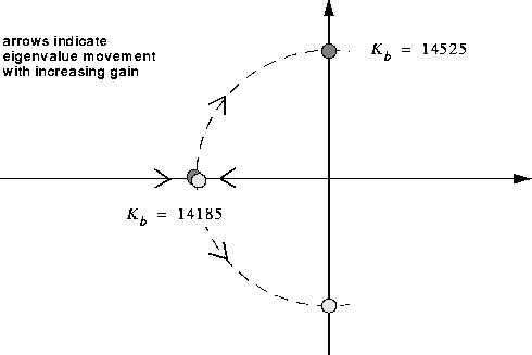
There is an interesting insight that emerges from the model at this stage. Consider figure 7, which shows the the positions of eigenvalues (drawn as small circles) as a function of two values of gain
We observe that the system is marginally stable for ![]() . On the other hand it is overdamped (non-volatile) for
. On the other hand it is overdamped (non-volatile) for ![]() ! Since real stock markets are volatile, i.e. underdamped (
! Since real stock markets are volatile, i.e. underdamped ( ![]() ), this suggests that there is some adaptive mechanism at work in the market to
keep
), this suggests that there is some adaptive mechanism at work in the market to
keep ![]() in the surprisingly narrow band
in the surprisingly narrow band ![]() , i.e. just under the instability border. We suggest that the mechanism is the
following: One one hand, agents jump in to trade on volatile movements. But by
their entry, they increase
, i.e. just under the instability border. We suggest that the mechanism is the
following: One one hand, agents jump in to trade on volatile movements. But by
their entry, they increase ![]() and thus volatility. On the
other hand they abstain when the market is too volatile (nervous market), thus
decreasing
and thus volatility. On the
other hand they abstain when the market is too volatile (nervous market), thus
decreasing ![]() and volatility.
and volatility.
The model is to be further elaborated, but first we will argue that from now on we may consider it to represent not a specific stock, but a ``composite stock'' composed of stocks from all firms listed on a stock exchange, such that the composite stock price is proportional to the stock exchange index. We make some assumptions in connection with this:
These assumptions mean that the composite stock p/e ratio (from
now on called an ``index'' or the ``price'' of the composite stock) will also
fluctuate around ![]() , with dynamics that are
similar to those for one category of stock. The difference is that a price shock
for one category of stock only, does not impact very strongly on the index.
, with dynamics that are
similar to those for one category of stock. The difference is that a price shock
for one category of stock only, does not impact very strongly on the index.
The aggregation step from one category of stock to an index is comparable to the earlier step of aggregating all agents into one composite agent. We uphold all variable and parameter names and numerical values introduced for the stock model, with the note that they now pertain to the index. By now we are ready to consider an augmented model as shown in figure 8.
Figure 8: Model incorporating long-term mood dynamics
Again we hold that model imperfections and approximations, and fluctuations
in demand for the composite stock implied by the index, is accounted for by a
zero mean noise process as introduced earlier. But we have for the time being
rescinded this stochastic excitation ![]() , since the dynamics to be
examined in this section will be shown not to depend upon being driven by an
external input. We will reintroduce the noise input later on.
, since the dynamics to be
examined in this section will be shown not to depend upon being driven by an
external input. We will reintroduce the noise input later on.
The additions to the model are indicated by the shaded area. Consider the
block in the upper right-hand corner. The instantaneous price increase rate is
an input to the block, a low pass filter with time lag ![]() of a one year magnitude. The rationale for this filter is that the increase rate
of ``optimism'' (or confidence, bullishness, positive ``animal spirits'' in the
terminology of Keynes) is assumed proportional to the long-term trend in index
increase. Hourly, daily, even weekly and (to some degree) monthly fluctuations
are disregarded; there is a sluggishness in market mood. Price rise has to be
persistent over a long time (years) before the market really picks up. On the
other hand, when the price culminates and starts falling, the market will need a
corresponding amount of time for such a change of affairs to sink in. The
increase rate in optimism is set equal to the markets' perception of the
long-term index increase rate. Optimism is given a numerical value, and a range
which is both positive and negative. (Thus pessimism corresponds to negative
optimism.)
of a one year magnitude. The rationale for this filter is that the increase rate
of ``optimism'' (or confidence, bullishness, positive ``animal spirits'' in the
terminology of Keynes) is assumed proportional to the long-term trend in index
increase. Hourly, daily, even weekly and (to some degree) monthly fluctuations
are disregarded; there is a sluggishness in market mood. Price rise has to be
persistent over a long time (years) before the market really picks up. On the
other hand, when the price culminates and starts falling, the market will need a
corresponding amount of time for such a change of affairs to sink in. The
increase rate in optimism is set equal to the markets' perception of the
long-term index increase rate. Optimism is given a numerical value, and a range
which is both positive and negative. (Thus pessimism corresponds to negative
optimism.)
By now it should be clear why it has been necessary to transit from an individual category of stock to an index: Market mood is a function of the behaviour of the aggregate of all stocks, not one category only.
In the absence of any perception of a long-term tendency for price to change
(i.e. a flat price level over a long period), the current level of optimism will
slowly erode to zero, through the factor ![]() . The argument for this is that the market will gradually forget its initial
mood and tend towards a neutral attitude (zero optimism or pessimism) if the
current mood is not maintained by a sustained increase or decrease in stock
price.
. The argument for this is that the market will gradually forget its initial
mood and tend towards a neutral attitude (zero optimism or pessimism) if the
current mood is not maintained by a sustained increase or decrease in stock
price.
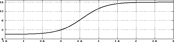
We may now try an experiment. We isolate the two blocks in the upper part of the figure from the model, input a rectangular price increase pulse, and observe the response in optimism given by this model. We assume a one-year (defined as 250 trading days) constant price increase rate pulse. This pulse, and the corresponding response in optimism, is illustrated in figure 9.
Figure 9: Optimism response to a pulse in price increase rate
Figure 10: Sigmoid function
The input pulse is not shown to scale. Parameter values for the simulation are chosen through a procedure described below. Note how optimism culminates after around 500 trading days (2 years). If we compare the time scales of figures 6 and 9, we observe a very large difference between the fast dynamics of the bandwagon loop, as opposed to the long-term mood loop. Thus we are dealing with a stiff system of differential equations.
To complete the explanation of the long-term mood loop, we now turn to the nonlinear sigmoid function . (The corresponding block in figure 8 is outlined in bold, to signify a nonlinear function.) The rationale for using the sigmoid is to account for upper and lower saturation in the system. The sigmoid function is shown in figure 10.
The function, including a gain ![]() introduced for convenience
(see figure 8),
outputs an additional demand component (measured in cash terms) which stems from
the long-term mood of the market. It may be positive or negative. This money
term translates into current additional composite stock demand
introduced for convenience
(see figure 8),
outputs an additional demand component (measured in cash terms) which stems from
the long-term mood of the market. It may be positive or negative. This money
term translates into current additional composite stock demand ![]() (``o'' for optimism) through division by the current index. Upper soft
saturation is assumed to make itself felt when the market is euphoric, i.e.
optimism is at a maximum. The will to spend money on additional stock
acquisition is there, but a very large amount of money has already been spent in
the stock market, and fresh cash and credit is getting scarce. At the other
extreme, when pessimism is at its maximum, agents holding stock are reluctant to
sell it at the going bottom price, since there is very little to gain. This
explains the lower saturation. The sigmoid function is expressed in the form
(``o'' for optimism) through division by the current index. Upper soft
saturation is assumed to make itself felt when the market is euphoric, i.e.
optimism is at a maximum. The will to spend money on additional stock
acquisition is there, but a very large amount of money has already been spent in
the stock market, and fresh cash and credit is getting scarce. At the other
extreme, when pessimism is at its maximum, agents holding stock are reluctant to
sell it at the going bottom price, since there is very little to gain. This
explains the lower saturation. The sigmoid function is expressed in the form
The parameters are:
![]() = The maximum saturation (asymptotic) value of
= The maximum saturation (asymptotic) value of ![]() is p. The minimum saturation is -n.
is p. The minimum saturation is -n.
![]() = The slope of
= The slope of ![]() for x=0. Thus
for x=0. Thus
![]() expresses the gain of
expresses the gain of ![]() for small excursions from a
neutral mood, into optimism or pessimism.
for small excursions from a
neutral mood, into optimism or pessimism.
Note that (7) has the
necessary property ![]() , i.e. a neutral market mood
results in zero additional demand. See also figure 10.
, i.e. a neutral market mood
results in zero additional demand. See also figure 10.
We have in this section introduced two first-order linear blocks and one non-linear relation, which together form the long-term mood loop. Figures 9 and 10 imply that numerical values for the parameters associated with this loop have been chosen. This is done in the following way: It is required that the system shall cycle regularly between euphoria and recession, but at this stage not allowing panics to occur. The maximum price (i.e. p/e ratio) is set to approx. 25, the minimum to approx. 5. Furthermore, a full cycle (which is at this stage not shortened by panics on the downswing, see next section), shall last 10 years (one year is defined as 250 trading days). It is demanded that upswings shall have an essentially exponential growth shape, and that downswings shall be faster than upswings. Based on these conditions, all parameters have been decided together, through educated guessing and a comprehensive simulation-based trial-and-error process.
With the resulting choice of parameters, the cycles look like in figure 11.
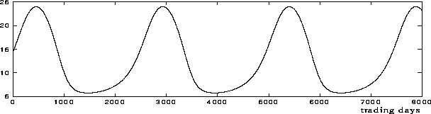
Figure 11: Cycles due to long-term mood dynamics
This is a stable limit cycle. In the next subsection we will see how this pattern is distorted by panics occurring near peak price levels, but we will also observe how this cycle remains an attractor that decides the fundamental long-run dynamics of the system. We emphasize that from this it follows that our model is not dependent upon a crash-and-subsequent-recovery mechanism for cycles to occur. The upswing is due to the spreading and self-reinforcing belief that ``if I get in now, I can cash in my investment with a profit at a later stage''. But the upswing sooner or later has to culminate at some level, when the perception has spread sufficiently that current prices have grown too high in relation to the sustainable value of the stock, and also due to increasing scarcity of additional money to invest in stocks. This reduces the growth rate of surplus demand and through this, the stock price growth rate. In the next round this reduces the growth rate in optimism, further reducing the demand growth rate, and so on. Optimism reaches a peak, and a feeling sooner or later overwhelms the optimistic mood of the upswing, and more stock is offered than demanded on the market. This further erodes optimism, and we are gradually into a downswing, which also needs time to build up momentum. This momentum causes the price to fall below sustainable value. But things will later pick up again when the earlier pessimistic mood is mostly forgotten, combined with a spreading recognition that the stock market is now generally undervalued. The upswing starts, and one cycle is completed. The period of a cycle is in the main decided by the inertia of market perception: It needs time to absorb a persistent tendency in price change, and it needs time to forget.
Note that our explanation for stock market cycles is a very psychological one. It has little connection with such other macroeconomic cycle explanations as Goodwin's business cycle model [6] where cycles are due to worker-capitalist struggle over output, or build-up of indebtedness and related financial fragility (Minsky's `financial instability hypothesis' [7], as modeled and simulated by Keen [8], or Andresen [9]).
Our purpose is not, however, to contest the validity of these other models-it is to focus on one specific approach that may be contain some truth together with other approaches. But we suggest that the mechanisms presented here have become relatively more important as the financial sector has grown in size and influence, as unions have lost power, as the focus of the media and thus public opinion, has turned from finance as an instrument for enhancing production, to the financial market as a place for playing games for profit; i.e. Keynes' ``Casino''.
The reader may at this stage object that the downswing predicted by our model is very slow and well-behaved. Where are the panics, which may erase a substantial part of an index in a single trading day? In the next section we will extend the model to account for this.
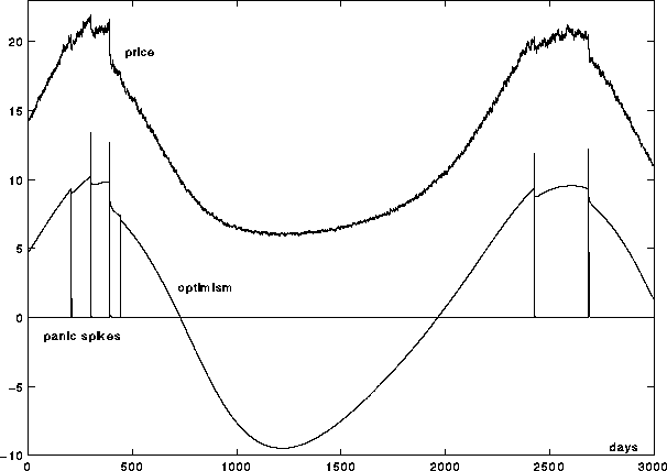
A modified model augmented with a panic mechanism is shown in figure 12.
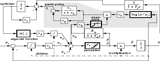
Figure 12: Model including panic mechanism
Figure 13: Two peaks with several crashes
The additions to the model in the previous subsection (figure 8) are indicated by the shaded area in figure 12.
We designate this ``the panic subsystem''. We note that this subsystem has
two inputs: The ratio ![]() , and relative price change
rate,
, and relative price change
rate, ![]() . The output is a negative pulse, designated
. The output is a negative pulse, designated ![]() in the figure. Such a pulse has the effect of abruptly reducing
optimism and thus the demand component
in the figure. Such a pulse has the effect of abruptly reducing
optimism and thus the demand component ![]() . We will explain the panic subsystem by starting to the right in the shaded
part of the figure, with the expression
. We will explain the panic subsystem by starting to the right in the shaded
part of the figure, with the expression ![]() . We have
. We have
Here the current price and time is ![]() , and the system starts with
, and the system starts with
![]() , i.e. price level equal to sustainable, ``fundamental'' value.
The logarithmic expression is equivalent to integrating relative price change
rate
, i.e. price level equal to sustainable, ``fundamental'' value.
The logarithmic expression is equivalent to integrating relative price change
rate ![]() , with initial value
, with initial value ![]() . Thus we have an expression that will be larger the further away from
sustainable value the price is. This expression is assumed to give a measure of
``wariness'' in the market. By this we mean that agents will on the average be
more sensitive to large downward blips in stock prices when the current prices
are much higher than sustainable value. The wariness factor is multiplied with
the output of a dead-zone block that ensures that only downward price blips
above a certain magnitude are passed on (i.e. noticed by the market), as
indicated by the graphics in that block. If prices are not too far away from
sustainable value, however, even large downward movements are not considered to
be danger signals. The filtered blips are passed on through a constant gain and
transfer function in parallel, as shown in the left part of the shaded area, and
then input to the optimism subsystem. The rationale for the transfer function,
which has low-pass character with a time lag
. Thus we have an expression that will be larger the further away from
sustainable value the price is. This expression is assumed to give a measure of
``wariness'' in the market. By this we mean that agents will on the average be
more sensitive to large downward blips in stock prices when the current prices
are much higher than sustainable value. The wariness factor is multiplied with
the output of a dead-zone block that ensures that only downward price blips
above a certain magnitude are passed on (i.e. noticed by the market), as
indicated by the graphics in that block. If prices are not too far away from
sustainable value, however, even large downward movements are not considered to
be danger signals. The filtered blips are passed on through a constant gain and
transfer function in parallel, as shown in the left part of the shaded area, and
then input to the optimism subsystem. The rationale for the transfer function,
which has low-pass character with a time lag ![]() (of magnitude a couple of weeks), is to account for medium-term memory in the
market of recent strong downward blips in an overvalued situation.
(of magnitude a couple of weeks), is to account for medium-term memory in the
market of recent strong downward blips in an overvalued situation.
At this stage it should be noted that it is not self-evident that this panic sub-system will actually lead to panics and crashes. We have just made some reasonable behavioural assumptions about wariness etc. for agents, and implemented them in the model. But we will see that panics will occur.
Now to the task of deciding values for the parameters, this time for the
panic sub-system. The procedure has been the same as described in the preceding
sections: back and forth between simulations, educated guesses, parameter
adjustments, new simulations. The resulting parameter value set is given at the
end of this paper. The variance and character of the stochastic noise process
![]() has also been decided as part of this selection process. Initially
white noise was tried, which is uncorrelated with itself between sampling
intervals (13 samples per trading day, i.e. a sample every half hour). This,
however, gave price movements that displayed distinct swings only from hour to
hour, but not over a couple of days. The white noise process was therefore
substituted with white noise filtered through a first order low-pass filter with
time lag = 3 trading days. This corresponds to a train of overlapping
exponentially-tailed pulses exciting the system, and gave autocorrelated price
dynamics over the week that (by visual inspection) resembled real-world index
movements well. We emphasize that panics and crashes occur whether one employs
white noise, correlated noise or a periodic pulse process to excite the system.
Figure 13
shows a simulation with the chosen parameter values. The simulations done were
quite time-consuming: We wanted to simulate over a couple of peaks, where the
time span is somewhat less than ten years = 2500 trading days, but where we also
had to account for price movements which may change significantly from half hour
to half hour. We thus had to use a stiff differential equation solver. To reduce
simulation time, simulations were started from a system state somewhat into the
peak (euphoric) phase of the first cycle. We observe from figure 13
that both the peak phases displays panics. Each panic is indicated by spikes,
four during the first euphoric phase, two during the second. These spikes are
the value of the variable
has also been decided as part of this selection process. Initially
white noise was tried, which is uncorrelated with itself between sampling
intervals (13 samples per trading day, i.e. a sample every half hour). This,
however, gave price movements that displayed distinct swings only from hour to
hour, but not over a couple of days. The white noise process was therefore
substituted with white noise filtered through a first order low-pass filter with
time lag = 3 trading days. This corresponds to a train of overlapping
exponentially-tailed pulses exciting the system, and gave autocorrelated price
dynamics over the week that (by visual inspection) resembled real-world index
movements well. We emphasize that panics and crashes occur whether one employs
white noise, correlated noise or a periodic pulse process to excite the system.
Figure 13
shows a simulation with the chosen parameter values. The simulations done were
quite time-consuming: We wanted to simulate over a couple of peaks, where the
time span is somewhat less than ten years = 2500 trading days, but where we also
had to account for price movements which may change significantly from half hour
to half hour. We thus had to use a stiff differential equation solver. To reduce
simulation time, simulations were started from a system state somewhat into the
peak (euphoric) phase of the first cycle. We observe from figure 13
that both the peak phases displays panics. Each panic is indicated by spikes,
four during the first euphoric phase, two during the second. These spikes are
the value of the variable ![]() defined in figure 12
(note: the scale on the ordinate axis pertains to price only, the other
variables are not shown to scale. For convenience,
defined in figure 12
(note: the scale on the ordinate axis pertains to price only, the other
variables are not shown to scale. For convenience, ![]() is shown, so the spikes turn up positive in figure 13).
is shown, so the spikes turn up positive in figure 13).
![]() is zero when the negative price blip is within the limit in the
dead-zone function, the ``background noise level'' that has to be surpassed
before the market is alarmed. If it is bigger than this limit, however, its
impact is decided by the value of the ``wariness factor'' (8), through
multiplication with this factor. The product, a negative pulse, is then
transmitted to the state that represents optimism, and this state is abruptly
reduced. The trajectory for the optimism state is also given in figure 13.
The abrupt decrease in optimism sets off a similarly abrupt decrease in demand,
which again transmits an amplified negative price blip to the input of the
dead-zone function. The loop is closed. We have positive feedback and a
mechanism to explain panics. More on this further below.
is zero when the negative price blip is within the limit in the
dead-zone function, the ``background noise level'' that has to be surpassed
before the market is alarmed. If it is bigger than this limit, however, its
impact is decided by the value of the ``wariness factor'' (8), through
multiplication with this factor. The product, a negative pulse, is then
transmitted to the state that represents optimism, and this state is abruptly
reduced. The trajectory for the optimism state is also given in figure 13.
The abrupt decrease in optimism sets off a similarly abrupt decrease in demand,
which again transmits an amplified negative price blip to the input of the
dead-zone function. The loop is closed. We have positive feedback and a
mechanism to explain panics. More on this further below.
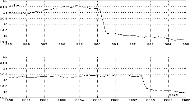
Figure 14 shows magnified portions of the two peak parts of the price curve. Note the time scale, a range of 300 trading days.
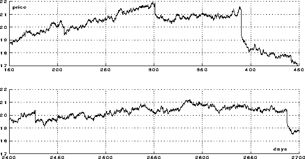
Figure 14: Two peak phases over 300 days
Figure 15: Zooming in on the 10 days around a panic
We observe that the two big panics during each of the two peak phases result in respectively a 12% and 6% price fall in a very short time. We have by this established that the panic mechanism works as predicted.
To get a clearer picture, we stretch the time axis even further, to get a glimpse of dynamics over a few days. The result is shown in figure 15. One day is divided into 13 sampling intervals. An initial downwards blip that is large enough to pass the dead-zone function, lasts only one sampling interval. The further downslide that may be observed for both peak phases, must therefore be a result of the aforementioned positive feedback loop.
If we ignore the panic events, and also trends, on the graphs in figures 14
and 15,
and inspect the price excursions under normal conditions, we note that prices
fluctuate between approx. ![]() to
to ![]() , which related to a level of 20 to 21, corresponds to
, which related to a level of 20 to 21, corresponds to ![]() to
to ![]() % . This is considered a realistic magnitude of
day-to-day volatility.
% . This is considered a realistic magnitude of
day-to-day volatility.
If we compare the two euphoric phases in figures 13 to 14, we observe that they are quite different in character. This can only stem from differences in the random noise process that excites the system, since all other conditions at the start of a euphoric phase are similar. We will now discuss this proposition more closely by presenting a series of simulation runs where the only parameter that is changed, is the ``seed'' integer initiating the random generator. This means that we have exactly the same dynamic system, starting from exactly the same initial state, but excited by different realizations of the same stochastic process. The results for eight such runs are given in figure 5.
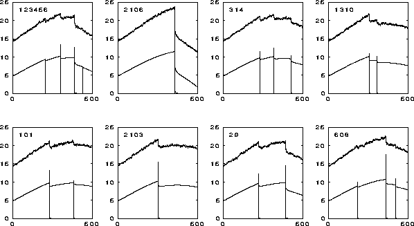
Figure 16: Euphoric phases for different seed integers
The integer listed on each graph is the corresponding seed integer. The upper left run is identical to the case already presented in figures 13 to 15. If we consider the eight graphs as a whole, the following observations may be made:
An early crash before price has gone to high, is a good thing in the sense that the crash will usually not be to big, as opposed to the case with seed = 2106, where a panic-free growth far above 20 results in a big 30% crash.
We also note that (small) crashes at an early stage contribute to reducing the danger of big crashes later. This, by the way, to some degree justifies the sometimes euphemistic term ``correction'' for crashes, so commonly used to calm market nerves.
Furthermore, we note that early crashes will not stop prices from continuing their rise later on, before culminating. This is due to the inertia of a general and still growing optimistic mood, a mood that needs more time and adversity to turn sour. On the other hand, if a big crash occurs when the euphoric phase is in a later and more mature stage, this crash will contribute to an earlier start of the inevitable general downslide. Generally, the presence of panics and ensuing crashes will lead to a shorter period for the long-term cycle than what is displayed by the panic-free limit-cycle model in figure 11.
To gain insight into the character of the euphoric phase disturbed by panics, consider the graphs for the optimism state (also shown in the plots in figure 16). Note the ``circular-saw-tooth'' appearance of these graphs. After a crash optimism growth is slower, if the crash happens on the upswing. If the crash happens on the downswing, the downwards slide is steeper afterwards.
As mentioned, the case with seed = 2106 displays the biggest crash of the
eight cases. At the bottom of the corresponding panic spike one may observe a
small decaying exponential tail. This accounts for the medium term memory in the
market of the crash, and stems from the low pass filter block with the
coefficients ![]() in figure 12.
Removing this block (and that memory effect), however, does not significantly
change system dynamics.
in figure 12.
Removing this block (and that memory effect), however, does not significantly
change system dynamics.
There are a couple of important mechanisms that are not incorporated in the current model. One phenomenon is ``rallying'', which takes place over a couple of days, or even several weeks. This phenomenon may occur as a consequence of a feeling after a recent panic or strong fall, that now is the time to buy cheap because stocks have fallen too much and will rise-which of course is a self-fulfilling prophecy if enough agents think this way. Or it may take place due to exogenous impulses, for instance an announcement of lower Central Bank interest rates, or an announcement of a what is believed to be a credible IMF rescue operation towards an important country or group of countries.
In terms of our model, this may be taken care of by introducing additional parallel feedback loops containing first- or second-order low pass transfer functions with time lags of a days/weeks magnitude, thus filling out the ``gap'' between the very short- and very long-term dynamics expressed by the corresponding loops in the current model. Such additional loops should enable the system to express swings over days and weeks, for instance rallying. Furthermore, one could look more closely into the modeling of exogenous impulses. In the current model, their impact all decay at the same rate, with a time constant of three days, and they arrive regularly (every half hour). A probably more realistic assumption is to let this noise be a Poisson process, thus generating impulses at irregular intervals, and more important-let these pulses decay at different rates, so that the model accounts for the fact that some news have more lasting influence on the market than other.
These suggested modifications will not, however, invalidate some insights and suggestions for further research that emerge from working with current model:
A final note: I wish to express my thanks to Dr. Steve Keen, the University of Western Sydney, for stimulating discussions, help and suggestions.
![]()
 |
 |
 |